I have watched a lot of tutorials and passed a bunch of courses about machine learning and AI before, but other than utilizing those methods on class assignments and a few of them for my master’s thesis, I didn’t have the chance to use machine learning and specifically deep learning in a long-term practical project. Fortunately, due to the need, I have in my research, I have started to study machine learning methods from scratch and this time more in-depth. According to a famous quote by Albert Einstein
“You do not really understand something unless you can explain it to your grandmother.”
It is quite important to be able to transfer your knowledge to others using plain and easily understandable descriptions which also helps to solidify your comprehension of the topic. So, I have decided to start a series of blog posts to build common machine learning algorithms from scratch in order to clarify these methods for myself and make sure I correctly understand the mechanics behind each of them.
Let me be clear from the very beginning: It’s all about fitting a function!
Consider we have a dataset containing the number of trucks crossing the border from Mexico to the U.S. through Ottay Messa port. Note that it’s just a subset of the entire inbound crossings dataset available on Kaggle. First of all, it’s always better to plot the data which may help us have some insight. To load the data from a .CSV file, we are going to use Pandas which is a well-known data analysis/manipulation python library. We can then plot the data using Matplotlib (another python library for data visualization).
df = pd.read_csv('./regression/dataset.csv')
x_training_set = pd.to_datetime(df.Date, infer_datetime_format=True).to_numpy()
y_training_set = df.Value.to_numpy()
number_of_training_examples = len(x_training_set)

#plot the raw data
fig, ax = plt.subplots(figsize=(8, 6))
year_locator = mdates.YearLocator(2)
year_month_formatter = mdates.DateFormatter("%Y-%m")
ax.xaxis.set_major_locator(year_locator)
ax.xaxis.set_minor_locator(mdates.YearLocator())
ax.xaxis.set_major_formatter(year_month_formatter)
ax.plot(x_training_set,y_training_set, ".")
fig.autofmt_xdate()
plt.show()
Note that in the original data, each value is corresponding to a month, so I mapped the date intervals into an integer representation.
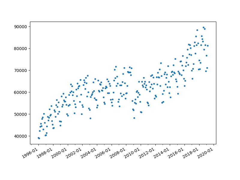
What we are observing here obviously is not an exact linear function, but for the sake of simplicity, we can model border crossings using a linear function! As we already know, the equation of a line is a below:
where m stands for the slope and c is the intercept on the y-axis. But we can have an infinite number of possible values for these parameters. Let’s look at some possible arbitrary lines with values [m=70,c=40000], [m=100,c=40000], [m=140,c=40000] represented with orange, green, and red colors respectively.
#plot arbitrary lines
def plot_line(ax, m,c,xMax):
    y0 = (1*m)+c
    ymax = (xMax*m)+c
    ax.plot([x_training_set[0],x_training_set[xMax-1]],[y0,ymax])

fig, ax = plt.subplots(figsize=(8, 6))
year_locator = mdates.YearLocator(2)
year_month_formatter = mdates.DateFormatter("%Y-%m")
ax.xaxis.set_major_locator(year_locator)
ax.xaxis.set_minor_locator(mdates.YearLocator())
ax.xaxis.set_major_formatter(year_month_formatter)
ax.plot(x_training_set,y_training_set, ".")
fig.autofmt_xdate()

plot_line(ax,70,40000,number_of_training_examples)
plot_line(ax,100,40000,number_of_training_examples)
plot_line(ax,140,40000,number_of_training_examples)
plt.show()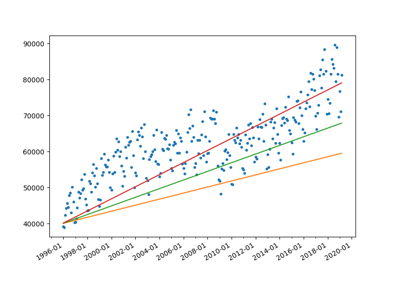
But, What are the parameter values we are choosing for our linear equation to properly fit our data points?
Analytical Approach to find the regression parameters
To find the proper fit for our data, basically, we have to minimize the average distance of the data points to our arbitrary line. In other words, we are finding the difference between the predicted value with the actual training data.
there are two ways to calculate the error:
Mean Squared Error (MSE): which considers the squared difference of the values.
Mean Absolute Error (MAE): which considers the absolute difference of the values.
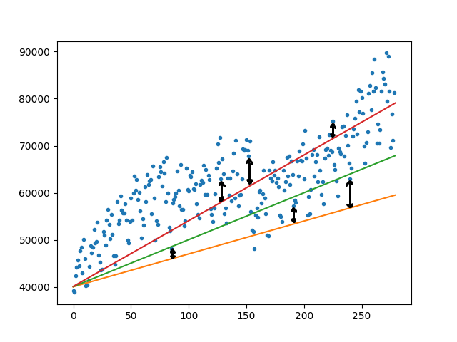
Note that we need to sum up these error values as positive numbers. Otherwise negative values will compensate for positive ones which will make our optimization problem impossible.
Our objective is to find our linear equation parameters m and c to minimize average error over all training set data (known as the cost function) defined below:
where n is the number of training examples. Now let’s explore the parameters space and plot the cost function to see what it looks like. for the MSE cost function, we have the parameters space-cost plot below
# visualize cost function
def line_equation(m,c,x):
    return (m*x)+ c

def cost_function(m,c,training_examples_x,training_examples_y):
    sum_of_errors = 0
    item_index = 0
    for example in training_examples_x:
        predicted_y = line_equation(m,c,item_index)
        sum_of_errors += (predicted_y - training_examples_y[item_index])**2
        #sum_of_errors += abs(predicted_y - training_examples_y[item_index])
        item_index+=1
    mse = (sum_of_errors / len(training_examples_x))
    return mse

fig = plt.figure()
fig.set_size_inches(8, 6)
ax = fig.add_subplot(projection='3d')
cost_func_x_points = []
cost_func_y_points = []
cost_func_z_points = []
for m in np.arange(-200,500,10):
    for c in np.arange(-10000,60000,200):
         cost = cost_function(m,c,x_training_set,y_training_set)
         cost_func_x_points.append(m)
         cost_func_y_points.append(c)
         cost_func_z_points.append(cost)
ax.scatter(cost_func_x_points, cost_func_y_points,
cost_func_z_points,c=cost_func_z_points,marker='.')
ax.set_xlabel('M')
ax.set_ylabel('C')
ax.set_zlabel('Cost')
plt.show()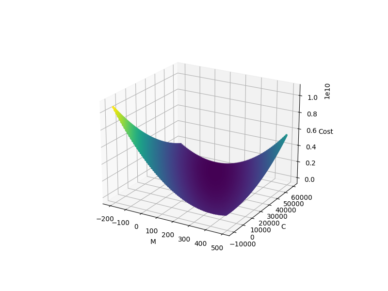
and for the MAE we have the plot below:
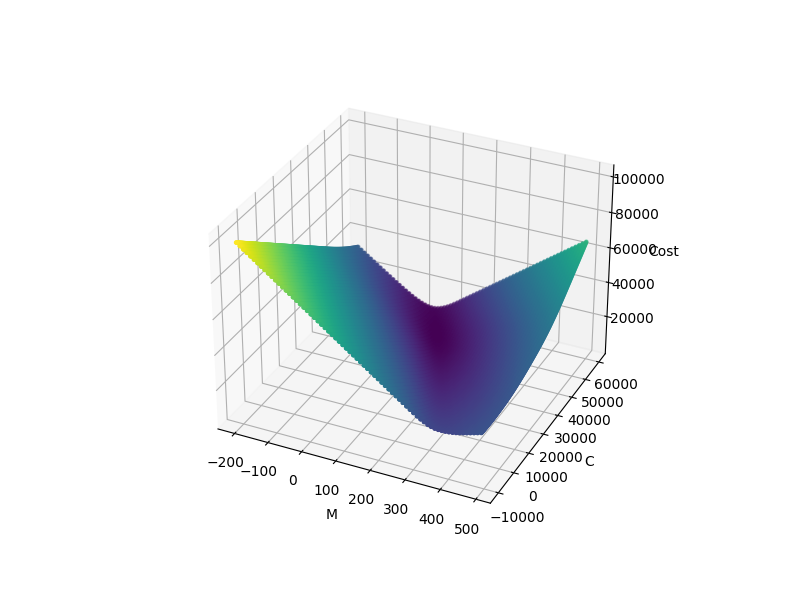
As you can see both these cost functions are convex and they just have one minimum point at the bottom of the slope(global minima). Then based on calculus, it means that if we could find the point that the derivative of this function is zero, we have found the optimal parameters for our model. We can simply use the equation below to find the parameters.
where X is the training features sample vector. Y is the output vector. and the result(theta) are the parameters for our regression model.
This equation is called a Normal Equation and you can find the math behind it here.
So let’s run it on our dataset and see how it works.
#linear equation using numpy
x_training_set_numbers = np.arange(0,len(x_training_set),1)
ones_vector = np.ones((len(x_training_set), 1))
x_training_set_numbers = np.reshape(x_training_set_numbers, (len(x_training_set_numbers), 1))
x_training_set_numbers = np.append(ones_vector, x_training_set_numbers, axis=1)
theta_list = np.linalg.inv(x_training_set_numbers.T.dot(x_training_set_numbers)) \
.dot(x_training_set_numbers.T).dot(y_training_set)
print(theta_list)

#visualize raw data with fitted line
fig, ax = plt.subplots(figsize=(8, 6))
year_locator = mdates.YearLocator(2)
year_month_formatter = mdates.DateFormatter("%Y-%m")
ax.xaxis.set_major_locator(year_locator)
ax.xaxis.set_minor_locator(mdates.YearLocator())
ax.xaxis.set_major_formatter(year_month_formatter)
ax.plot(x_training_set,y_training_set, ".")
fig.autofmt_xdate()
plot_line(ax,theta_list[1],theta_list[0],number_of_training_examples)
plt.show()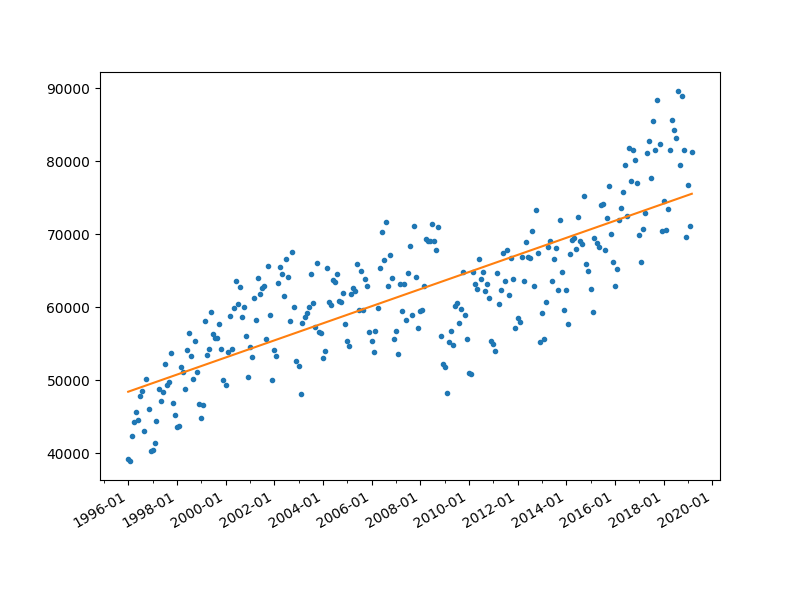
[48326.215617 97.55941938]Model Evaluation
Now that we have fit a line on our data, are we done? Nope!
We need to evaluate the model utilizing different metrics and plots to make sure the model we proposed would generalize well on new data.
To evaluate a model there are several metrics we can use.
1- MSE (Mean Squared Error)
2- MAE (Mean Absolute Error)
These two metrics mentioned above, have the exact same definition we had in defining the cost functions. The main difference between these two is MSE penalizes prediction errors heavily in comparison to MAE. Generally, we want these scores to be as close as possible to zero.
mse_value = 0
mae_value = 0
m  = theta_list[1]
c = theta_list[0]
for sample_x in range(0,number_of_training_examples):
    predicted_y =  m * sample_x + c
    sample_y = int(y_training_set[sample_x])
    mse_value += (predicted_y - sample_y)**2
    mae_value += abs(predicted_y - sample_y)
print(f"Mean Squared Error: {mse_value//number_of_training_examples}\n")
print(f"Mean Absolute Error: {mae_value//number_of_training_examples}\n")
3- R-Squared Score
In terms of regression evaluation, the R-Square score or R2 score is one of the most useful ones. It indicates how much variance of the data is explained by the model. In other words, it indicates how close is the data point to the fitted line. R2 score is defined as below:
R2 score must be a number between 0 and 1. In regression modeling, we aim to maximize the R2 score toward 1 as much as possible. Note that if the R2 score is a negative value, it’s indicating that something is wrong with the modeling or implementations.
4- Residual Plot
Also, it’s crucial to plot residuals to see if linear regression is a good choice to model our data. In regression, residual is the difference between the actual value and the predicted value. Residual points have to distribute equally along the horizontal axis. Otherwise, the model is not performing well and probably it’s not reliable enough.
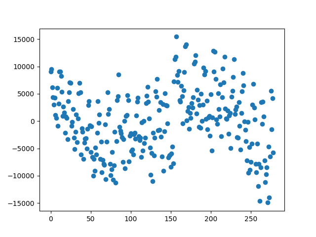
In the figure above, except at the beginning and the end of the plot, in which residuals have greater values, residuals are somehow randomly distributed. Generally, for a good linear regression model, data points in this plot must be as close as possible to the horizontal axis, and also they have to be uniformly distributed along the plot.
Code Refactoring
although what we have done till here is working, but it’s quite a mess in terms of performance and cleanness. Accordingly, I’m gonna wrap the implementation in a class called LinearRegressor as follows.
import numpy as np

class LinearRegressor:
    """Simple linear regression model"""
    def __init__(self, loss='MSE'):
        self.coeff = []

        def MSE(y_predicted, y_target):
            return ((y_target-y_predicted)**2).mean()

        def MAE(y_predicted, y_target):
            return (abs(y_target-y_predicted)).mean()

        if loss == 'MSE': self.calculate_loss = MSE
        elif loss == 'MAE': self.calculate_loss = MAE
        else: self.calculate_loss = MSE

    def __add_bias(self, x):
        one = np.ones((len(x),1))
        return np.append(one, x, axis=1)

    def fit(self, x, y):
        x = self.__add_bias(x)
        self.coeff = np.linalg.inv(x.T.dot(x)).dot(x.T).dot(y)

    def predict(self, x):
        x = self.__add_bias(x)
        return x.dot(self.coeff)
Test for simple regression
# simple linear regression
x = np.array([1,2,3,4,5,6]).reshape(-1, 1)
y = np.array([2,4,6,8,14,12])

model = LinearRegressor(loss="MAE")
model.fit(x,y)
predicted_y = model.predict(x)
print(f'Coefficients: {model.coeff}')
print(f'Predicted values: {predicted_y}')
print(f'Loss: {model.calculate_loss(predicted_y,y)}')
Coefficients: [-0.53333333 2.34285714]
Predicted values: [ 1.80952381 4.15238095 6.4952381 8.83809524 11.18095238 13.52380952]
Loss: 1.00317460317459907Test for multiple regression
#multiple regression
x = np.array([[1,2],[3,4],[5,6],[7,6],[9,8],[11,6]])
y = np.array([2,4,6,8,14,12])

model = LinearRegressor(loss="MAE")
model.fit(x,y)
predicted_y = model.predict(x)
print(f'Coefficients: {model.coeff}')
print(f'Predicted values: {predicted_y}')
print(f'Loss: {model.calculate_loss(predicted_y,y)}')
Coefficients: [-1.36363636 0.81818182 0.77272727]
Predicted values: [ 1. 4.18181818 7.36363636 9. 12.18181818 12.27272727]
Loss: 0.939393939393931822Great! Note that to be able to multiply a 1-d NumPy array with another array we need to use reshape() function, or change the array to an array of 1×1 arrays!
Also, to consider biases in this class, we have to add a column with value of 1 to each datapoint in the dataset which is done in both fit() and predict() function by calling the __add_bias() function.
Let’s run it on the dataset we prepared in beginning of the post and see if it leads to the same result.
import pandas as pd
import numpy as np
from linearregressor import LinearRegressor

df = pd.read_csv('./regression/dataset.csv')
x_raw = pd.to_datetime(df.Date, infer_datetime_format=True).to_numpy()
y = df.Value.to_numpy()

x = np.arange(0,len(x_raw),1)

model = LinearRegressor()
model.fit(x.reshape(-1, 1),y)
predicted_y = model.predict(x)

print(f'Coefficients: {model.coeff}')
print(f'Loss: {model.calculate_loss(predicted_y,y)}')
[48326.215617 97.55941938]
Loss: 35035066.896423854Polynomial Regression
Based on the visualizations we had in the very first steps, we could clearly see that what we are dealing with is not a linear function. Accordingly, we have to try a more flexible function to fit to our data. To do so, what we can do is adding polynomial features created from the original features.
x = np.arange(0,len(x_raw),1).reshape(-1, 1)
x2 = (x)**(2)
x = np.append(x2, x , axis=1)
print(x.shape)
(279, 2)Then feed the new feature set to the linear regressor model.
model = LinearRegressor()
model.fit(x,y)
predicted_y = model.predict(x)

print(f'Coefficients: {model.coeff}')
print(f'Loss: {model.calculate_loss(predicted_y,y)}')
Coefficients: [4.94483798e+04 8.74345493e-02 7.32526147e+01]
Loss: 34777741.55225808Good! it could decrease the loss value! By the same way we can add higher order polynomials.
x = np.arange(0,len(x_raw),1).reshape(-1, 1)
x2 = (x)**(2)
x3 = (x)**(3)
x4 = (x)**(4)
x = np.append(x2, x , axis=1)
x = np.append(x3, x , axis=1)
x = np.append(x4, x , axis=1)
print(x.shape)

model = LinearRegressor()
model.fit(x,y)
predicted_y = model.predict(x)

print(f'Coefficients: {model.coeff}')
print(f'Loss: {model.calculate_loss(predicted_y,y)}')
279, 4)
Coefficients: [ 4.13050845e+04 -4.22457826e-07 7.56166532e-03 -3.07680331e+00
4.26784643e+02]
Loss: 24975813.83882587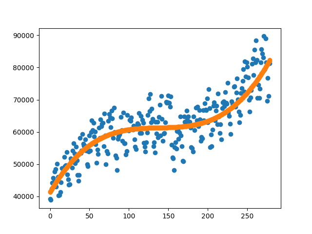
Leave a Reply