Implementing a real-life example of things that I’m trying to comprehend, is the most exciting part of the learning process for me. It gives me a chance to encounter with dark corners and pitfalls. Accordingly, I’m going to briefly write up about a recent project I have done on simple audio classification using machine learning. In this project, I will implement a machine learning model to classify fire alarm, vacuum cleaner, music, and silence sounds.
Data Collection
Every machine learning pipeline starts with a data collection and prepration stage. I have collected audio samples in .WAV format using the Audacity desktop application on the windows with 44.1 khz sample rate. Note that we consider silence as a seperate class. Each sample is roughly 30 seconds. For music, fire alarm, and vacuum cleaner, I recorded samples from online audio. For each class, I collected at least 20 samples, in different sessions with different ambient noise and background to have a more diverse dataset which helps our model to be more generalized and robust.
For loading audio samples, preprocessing, and feature extraction I have used a popular python library called Librosa. It seems that intalling Librosa using pip is problematic due to unknown reasons. Accordingly, I highly recommend to install it using Conda to avoid any inconsistency and hassles on Windows.
import os
import numpy as np
import matplotlib.pyplot as plt
import librosa
import librosa.display
from scipy.fft import rfft, rfftfreq
import cv2
import pickle

from sklearn.model_selection import cross_val_score
from sklearn.svm import SVC
from sklearn.metrics import classification_report, accuracy_score
from sklearn.metrics import ConfusionMatrixDisplay

ROOT_DIR = 'C:/Users/amiri/Desktop/demo/dataset/'
SAMPLING_RATE = 44100 #it's consistent over the entire dataset recordings

def get_all_directories(root_path):
    dirs = os.listdir(root_path)
    dirs = [dir for dir in dirs if os.path.isdir(root_path+dir)]
    return dirs

def get_all_files(path):
    files = os.listdir(path)
    files = [file for file in files if os.path.isfile(path+file)]
    return files

def load_all_audio_files(root_path, duration=30):
    files = get_all_files(root_path)
    file_samples = []
    for file in files:
            samples, sampling_rate = librosa.load(root_path+file,
             sr=None, mono=True, offset=0.0, duration=duration)
            file_samples.append(samples)
    return file_samples

dataset = {}
for audio_class in get_all_directories(ROOT_DIR):
    dataset[audio_class] = load_all_audio_files(ROOT_DIR + audio_class+'/')
    print(f"number of {audio_class} samples: {len(dataset[audio_class])}")
Now let’s visualize the samples and take a look at the audio signals to have an intuition about different audio shapes and variations.
fig, axs = plt.subplots(4,figsize=(8, 5), sharex=True,
constrained_layout = True)
fig.suptitle('Time-Amplitude Visualizaition')

ax_index = 0
sample_index = 0
for audio_class in dataset:
    axs[ax_index].title.set_text(f'{audio_class} Audio Sample \n')
    librosa.display.waveshow(dataset[audio_class][sample_index],
     sr=SAMPLING_RATE, ax = axs[ax_index])
    ax_index+=1
plt.show()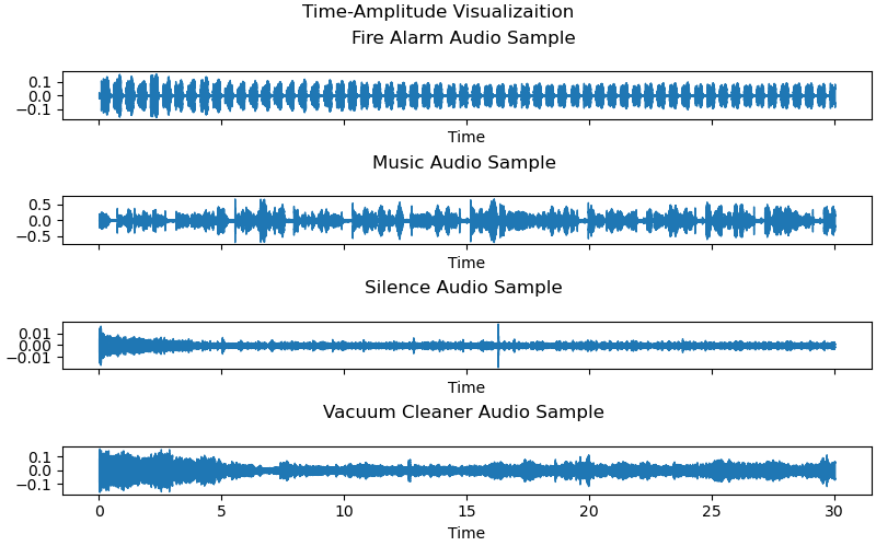
Domain Specific Features
Based on the sound waves visualized above. We may be able to use some time-domain features like: number of zero crossings, mean flatness, maximum amplitude, minimum amplitude, kurtosis and skewness.
def get_zero_crossing_features(wave_sample):
    crossings = np.nonzero(librosa.zero_crossings(wave_sample))[0]
    number_of_zero_crossings = len(crossings)
    mean_zero_crossing_rate = librosa.feature.zero_crossing_rate(wave_sample).mean()

    return number_of_zero_crossings, mean_zero_crossing_rate

def get_mean_flatness(audio_sample):
    return librosa.feature.spectral_flatness(y=audio_sample).mean()

def get_time_domain_features(audio_sample):

    mean_flatness = get_mean_flatness(audio_sample)
    number_of_zero_crossings , mean_zero_crossing_rate = get_zero_crossing_features(audio_sample)
    max_ampl = audio_sample.max()
    min_ampl = audio_sample.min()
    variance_ampl = np.var(audio_sample)
    kurtosis = sc.stats.kurtosis(audio_sample)
    skewness = sc.stats.skew(audio_sample)
    return number_of_zero_crossings, mean_zero_crossing_rate,
     max_ampl, min_ampl, variance_ampl, mean_flatness,kurtosis, skewness

data = []
labels = []
for audio_class in dataset:
    for audio_sample in dataset[audio_class]:
        time_domain_features = list(get_time_domain_features(audio_sample))
        feature_set = np.concatenate([time_domain_features])
        labels.append(audio_class)
        data.append(feature_set)

data = np.array(data)
labels = np.array(labels)
Now that we constructed the feature set, we can go ahead and feed them into different classification methods and see if they can correctly classify audio recordings!
xtrain, xtest, ytrain, ytest = train_test_split(data, labels, test_size=0.3, shuffle=True)
svm_rbf = SVC()
svm_rbf.fit(xtrain, ytrain)
svm_rbf_scores = cross_val_score(svm_rbf, xtrain, ytrain, cv=10)
print('Average Cross Validation Score from Training:',
 svm_rbf_scores.mean(), sep='\n', end='\n\n\n')


svm_rbf_ypred = svm_rbf.predict(xtest)
svm_rbf_cr = classification_report(ytest, svm_rbf_ypred)

print('Test Statistics:', svm_rbf_cr, sep='\n', end='\n\n\n')

svm_rbf_accuracy = accuracy_score(ytest, svm_rbf_ypred)
print('Testing Accuracy:', svm_rbf_accuracy)

fig, ax = plt.subplots(figsize=(5,5))
ConfusionMatrixDisplay.from_estimator(svm_rbf, xtest, ytest,
 ax = ax, cmap='RdYlGn')
plt.show()
and Voila!
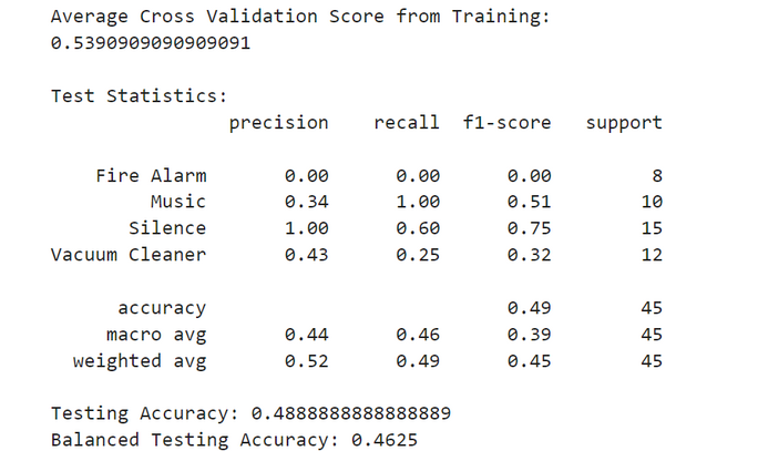
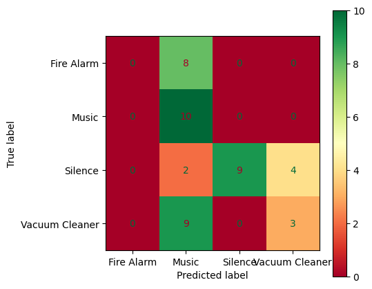
Disappointing! Isn’t it?!
But, why the model showed such a poor classification result? First of all, we should take a step back and look at the dataset itself to find a clue.
import pandas as pd
dataframe = pd.DataFrame.from_records(data)
dataframe.describe()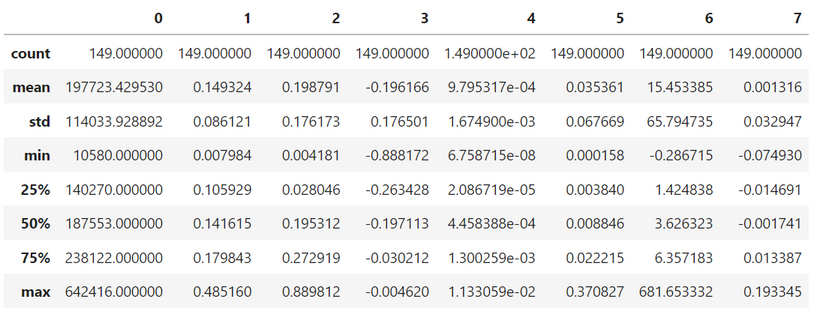
We can clearly see that the features have different value ranges, which could drastically reduce the model accuracy if the machine learning model works based on distance between data points! (which in our case SVM classifier does.)
Accordingly, a StandardScaler is added to the pipeline to normalize data. Let’s see if it can improve the accuracy or not.
from sklearn.model_selection import train_test_split
from sklearn.pipeline import Pipeline
from sklearn.svm import SVC
from sklearn.preprocessing import StandardScaler
from sklearn.metrics import balanced_accuracy_score

xtrain, xtest, ytrain, ytest = train_test_split(data, labels, test_size=0.3, shuffle=True)
svm_rbf = Pipeline([('scaler', StandardScaler()), ('svc', SVC())])
svm_rbf.fit(xtrain, ytrain)
svm_rbf_scores = cross_val_score(svm_rbf, xtrain, ytrain, cv=10)
print('Average Cross Validation Score from Training:',
 svm_rbf_scores.mean(), sep='\n', end='\n\n\n')


svm_rbf_ypred = svm_rbf.predict(xtest)
svm_rbf_cr = classification_report(ytest, svm_rbf_ypred)

print('Test Statistics:', svm_rbf_cr, sep='\n', end='\n\n\n')

svm_rbf_accuracy = accuracy_score(ytest, svm_rbf_ypred)
print('Testing Accuracy:', svm_rbf_accuracy)

balanced_accuracy = balanced_accuracy_score(ytest, svm_rbf_ypred)
print('Balanced Testing Accuracy:', balanced_accuracy)


fig, ax = plt.subplots(figsize=(5,5))
ConfusionMatrixDisplay.from_estimator(svm_rbf, xtest, ytest,
 ax = ax, cmap='RdYlGn')
plt.show()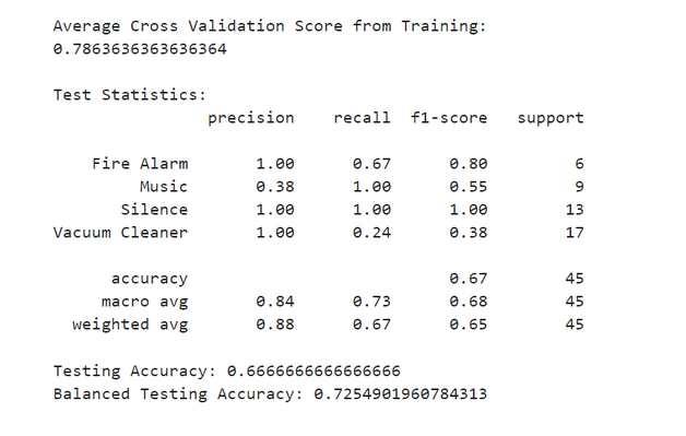
Well! We could improve the model accuracy about twenty percent just by normalizing features!
But, the result is still not satisfactory. We can try adding more features, or trying other models to see if we can improve the work. To add more features we can convert the audio samples to frequency-domain and see if we can extract more meaningful information and features. It’s easy to change audio signals to frequency-domain in Librosa and also Scipy libraries using Fast Fourier Transform. It’s basically a method to transform discrete spacial data to a discrete frequency histogram. In other words it reveals the frequencies distribution of the signal.
from scipy.fft import rfft, rfftfreq

def Get_RFFT(audio_sample):
    N = len(audio_sample)
    yf = rfft(audio_sample)
    xf = rfftfreq(N, 1 / SAMPLING_RATE)
    return xf, yf

fig, axs = plt.subplots(4,figsize=(8, 5), sharex=True,
constrained_layout = True)
fig.suptitle('Frequency-Domain Visualizaition')

ax_index = 0
sample_index = 0
for audio_class in dataset:
    audio_sample = dataset[audio_class][sample_index]
    axs[ax_index].title.set_text(f'{audio_class} \n')
    audio_sample_xf, audio_sample_yf = Get_RFFT(audio_sample)
    axs[ax_index].plot(audio_sample_xf, np.abs(audio_sample_yf))
    ax_index+=1

plt.show()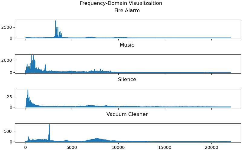
The figure above, illustrates the frequencies in one randomely chosen sample of each class. We can see each audio sample contains different frequencies which we can be leveraged as a new feature. But, what we do instead, is sliding a window of a fixed size on the original signal, and extract frequency distribution on each window using FFT. Eventualy, by column-wise concatenation of each FFT output, we will have a two-dimentional array of frequencies in time, which is called a Spectrogram. Fortunately, Librosa library made our life easier and provided neat functions to extract and visualize the spectrogram of a signal.
import matplotlib.pyplot as plt

FFT_SIZE = 1024*4
WINDOW_SIZE = FFT_SIZE//2

fig, axs = plt.subplots(4,figsize=(15, 15), sharex=True,
constrained_layout = True)
fig.suptitle('Frequency-Domain Visualizaition')


ax_index = 0
sample_index = 15
for audio_class in dataset:
    audio_sample = dataset[audio_class][sample_index]
    S = np.abs(librosa.stft(audio_sample,n_fft=FFT_SIZE,win_length=WINDOW_SIZE))
    power_fft = librosa.amplitude_to_db(S,ref=np.max)
    axs[ax_index].title.set_text(f'{audio_class} \n')
    img = librosa.display.specshow(power_fft, y_axis='log', x_axis='time',
                                   ax=axs[ax_index],sr = SAMPLING_RATE)
    axs[ax_index].set_title(f'{audio_class} Power spectrogram')
    fig.colorbar(img, ax=axs[ax_index], format="%+2.0f dB")
    ax_index+=1

plt.show()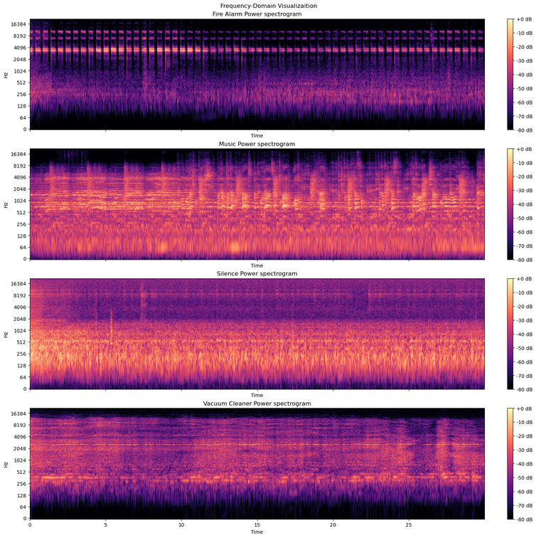
As shown in the figure above, Spectrogram is actually an image containing the changes in frequency over time. Now, we have a rich feature in frequency-domain, we are gonna flatten the 2-D sepctrogram array to a 1-d array and concatenate them to the time-domain features. Also, to reduce the spectrogram size, I have treated the spectrogram as an image and resized it using OpenCv.
data = []
labels = []
num_freq_bins=32
num_time_bins=256
for audio_class in dataset:
    for audio_sample in dataset[audio_class]:

        time_domain_features = list(get_time_domain_features(audio_sample))

        spectro = np.abs(librosa.stft(audio_sample,n_fft=FFT_SIZE,win_length=WINDOW_SIZE))
        power_spectro = librosa.amplitude_to_db(spectro,ref=np.max)
        binned_power_spectro = cv2.resize(power_spectro[:,:],(num_time_bins,num_freq_bins))

        feature_set = np.concatenate([binned_power_spectro.ravel(), time_domain_features])
        data.append(feature_set)
        labels.append(audio_class)


data = np.array(data)
labels = np.array(labels)
data.shape
Finally, the dataset is fed into the SVM classifier with results shown below.
from sklearn.model_selection import train_test_split
from sklearn.pipeline import Pipeline
from sklearn.svm import SVC
from sklearn.preprocessing import StandardScaler
from sklearn.metrics import balanced_accuracy_score
print('\n')

xtrain, xtest, ytrain, ytest = train_test_split(data, labels, test_size=0.3, shuffle=True)
svm_rbf = Pipeline([('scaler', StandardScaler()),('svc', SVC())])
svm_rbf.fit(xtrain, ytrain)
svm_rbf_scores = cross_val_score(svm_rbf, xtrain, ytrain, cv=10)
print(f'10-Fold CV Score :{svm_rbf_scores.mean():.3f} ± {svm_rbf_scores.std():.3f}',
      sep='\n', end='\n\n\n')


svm_rbf_ypred = svm_rbf.predict(xtest)
svm_rbf_cr = classification_report(ytest, svm_rbf_ypred)

print('Test Statistics:', svm_rbf_cr, sep='\n', end='\n')

svm_rbf_accuracy = accuracy_score(ytest, svm_rbf_ypred)
print('Testing Accuracy:', svm_rbf_accuracy)

balanced_accuracy = balanced_accuracy_score(ytest, svm_rbf_ypred)
print('Balanced Testing Accuracy:', balanced_accuracy)


fig, ax = plt.subplots(figsize=(5,5))
ConfusionMatrixDisplay.from_estimator(svm_rbf, xtest, ytest,
 ax = ax, cmap='RdYlGn')
plt.show()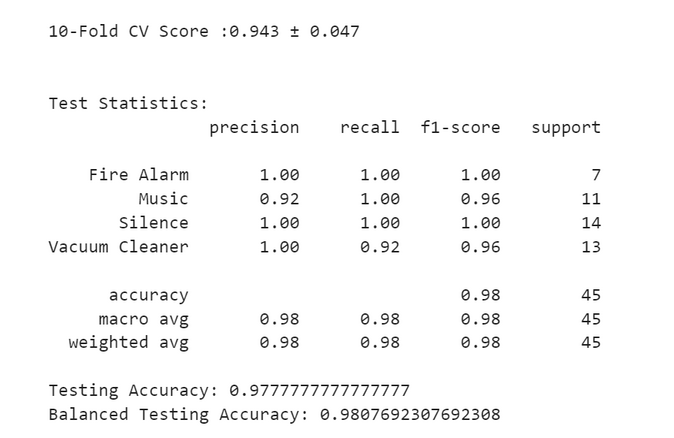
Real-Time Audio Classification
Till now, we have used 30-second audio samples. But this duration is too much if we are aiming to use the model in a real-time situation like smart-home applications. Accordingly, first of all we have to decrease the sample sizes and try to detect the events in a smaller time window. One way around it is to slide a fixed window size on the original audio samples and create another dataset out of the extracted windows. If we slide the window without any overlap then we can use the same pipeline as we have developed before. Since we may lose some of the event data which lies between two consecutive frames, it’s better to have at least a 50 percent overlap between consecutive frames. But, it’s a bit tricky! Because if we introduce overlapping frames in the dataset, then the evaluation process may shows a bloated result. In other words, the test may contains the frames which have seen before by the model in the training set! Accordingly, it will lead to an unreliable model performance evaluation.
If we had enough data, then we could simply seperate train and test samples before applying the sliding window on them. But here, we utilize a method called BlockingTimeSeriesSplit which is a well-known method for time-series cross-validation split. more details here ,and here.
Ok then, first of all, we need to extract the frames using function defined below.
def get_windows(wave_sample, dataclass, sampling_rate, window_size_seconds=1, overlap = 0.5):
    sub_samples_data = []
    labels = []
    samples_per_window = int(sampling_rate) * window_size_seconds
    window_shift_by = int((1-overlap) * samples_per_window)
    window_index = 0

    while not ((window_index + samples_per_window)>wave_sample.shape[0]):
        sub_samples_data.append(wave_sample[window_index: window_index + samples_per_window])
        window_index+=window_shift_by

    labels.extend([dataclass]  * len(sub_samples_data))
    return sub_samples_data, labels
data = {}

for audio_class in dataset:
    class_sub_features = []
    for audio_sample in dataset[audio_class]:
        sub_samples_data, sub_samples_labels = get_windows(wave_sample = audio_sample,
                                               dataclass = audio_class,
                                               sampling_rate = SAMPLING_RATE
                                              , window_size_seconds=2)
        for i in range(len(sub_samples_data)):
            time_domain_features = list(get_time_domain_features(sub_samples_data[i]))


            spectro = np.abs(librosa.stft(sub_samples_data[i],n_fft=FFT_SIZE,
            win_length=WINDOW_SIZE))
            power_spectro = librosa.amplitude_to_db(spectro,ref=np.max)
            binned_power_spectro = cv2.resize(power_spectro[:,:],(num_time_bins,num_freq_bins))

            time_feauture_set = [time_domain_features,]
            freq_feature_set = [binned_power_spectro.ravel(),]


            final_feature_set =  time_feauture_set + freq_feature_set
            feature_set = np.concatenate(final_feature_set)
            class_sub_features.append(feature_set)
    data[audio_class] = class_sub_features
Feature extraction process is the same as before, but here we added an inner loop to slide a window on each audio sample and extract the features for each frame to build the new dataset.
Then the dataset is splitted using the Blocking TimeSeries Split method. Note that the dataset shouldn’t get shuffled before this process.
class BlockingTimeSeriesSplit():
    def __init__(self, n_splits, test_size=0.3, hop=2):
        self.n_splits = n_splits
        self.test_size = test_size
        self.hop = hop

    def get_n_splits(self, X, y, groups):
        return self.n_splits

    def split(self, X, y=None, groups=None):
        n_samples = len(X)
        k_fold_size = n_samples // self.n_splits
        indices = np.arange(n_samples)

        for i in range(self.n_splits):
            start = i * k_fold_size
            stop = start + k_fold_size
            mid = int((1-self.test_size) * (stop - start)) + start
            yield indices[start: mid], indices[mid + self.hop: stop]
blocking_timeseries_split = BlockingTimeSeriesSplit(n_splits=30, test_size=0.3, hop=2)

x_test_groups = []
x_train_groups = []

y_test_groups = []
y_train_groups = []
for audio_class in data:
    class_data = np.array(data[audio_class])
    for train_index, test_index in blocking_timeseries_split.split(class_data):

       #print("TRAIN:", train_index, "TEST:", test_index)
       x_train, x_test = class_data[train_index], class_data[test_index]
       y_train = [audio_class]  * len(x_train)
       y_test = [audio_class]  * len(x_test)
       x_test_groups.extend(x_test)
       x_train_groups.extend(x_train)

       y_test_groups.extend(y_test)
       y_train_groups.extend(y_train)

x_test_groups = np.array(x_test_groups)
x_train_groups = np.array(x_train_groups)

y_test_groups = np.array(y_test_groups)
y_train_groups = np.array(y_train_groups)
Finally, the training set and testing set are fed to the machine learning pipeline for training and evaluation.
model = Pipeline([('scaler', StandardScaler()),('svc', SVC())])

model.fit(x_train_groups, y_train_groups)
model_scores = cross_val_score(model, x_train_groups, y_train_groups,
 cv=10,scoring="balanced_accuracy")

print(f'10-Fold CV Score :{model_scores.mean():.3f} ± {model_scores.std():.3f}',
 sep='\n', end='\n\n')

model_ypred = model.predict(x_test_groups)
model_cr = classification_report(y_test_groups, model_ypred)

print('Test Statistics:', model_cr, sep='\n', end='\n\n')

model_accuracy = accuracy_score(y_test_groups, model_ypred)
print(f'Testing Accuracy:{model_accuracy:.3f}')


balanced_model_accuracy = balanced_accuracy_score(y_test_groups, model_ypred)
print(f'Balanced Testing Accuracy:{balanced_model_accuracy:.3f}')

fig, ax = plt.subplots(figsize=(5,5))
ax.grid(False)
ConfusionMatrixDisplay.from_estimator(model, x_test_groups, y_test_groups,ax = ax,
 cmap='Greens')
plt.show()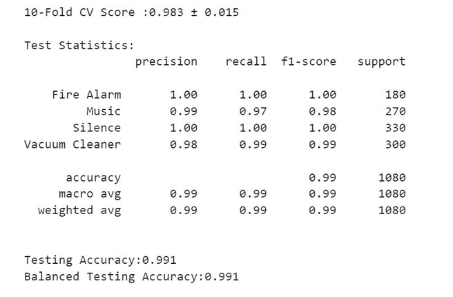
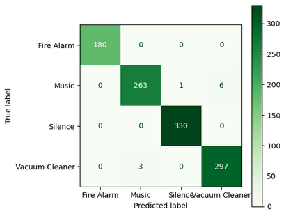
Sounds Great!
Real-Time Audio Classification Live Demo
Now let’s use the model in a real-time application and see if it works as expected! To do so, first of all we need to save the trained model using the python pickle object serialization library.
import pickle
filename = 'audio_classifier.ml'
pickle.dump(model, open(filename, 'wb'))
Next, we have to read the microphone data using pyaudio python library by instantiating a PyAudio object and open it with same sampling frequency we recorded the sample audio with.
import pyaudio
SAMPLING_RATE  = 41000
CHUNK_SIZE   = SAMPLING_RATE // 10

py_audio = pyaudio.PyAudio()
input_audio_stream = py_audio.open(format=pyaudio.paFloat32,
channels=1, rate=SAMPLING_RATE, input=True,
frames_per_buffer=CHUNK_SIZE)
Note that the pyaudio buffers up the samples from the microphone and returns them whenever it reached the threshold parameter frames_per_buffer as a whole.
Now we can read the last chunk of data in a loop. Note that this method of reading input data which is called Blocking, is deprecated in real-world implementation since if the processing happens in a same thread as reading, it will create a lag between each read and eventauly will led to missing parts of the actual audio. To work around this issue, data should be read in a seperate thread and process in a different thread (typical producer/consumer problem). But for the sake of simplicity we don’t get into that here.
try:
    while True:
        # reading and converting pyaudio input to np array
        raw_data_chunk = np.fromstring(input_audio_stream.read(CHUNK_SIZE),dtype=np.float32)


        cv2.waitKey(1)

except KeyboardInterrupt:
    input_audio_stream.stop_stream()
    input_audio_stream.close()
You might think if we add the machine learning model after reading audio, we should be done! In fact it will somehow work, but the problem is data is read every 2 seconds and discarded after we have processed it! So, what if an event happened between two consecutive audio signal chunks?
To solve this issue we have to decrease the input chunk size and buffer the input data, just like we did in training phase. Then we can slide a fixed-size window on the buffer and feed the window content to the machine learning pipeline.
To do so, I have written a class name WindowedBuffer as below:
import numpy as np

class WindowedBuffer1D:

    def __init__(self, buffer_size:int, window_size:int, window_loc = "center"):

        self.buffer_size = buffer_size
        self.window_size = window_size
        self.buffer = None
        self.chunk_number = 0
        if window_loc == "center" or None:
            self.window_start_loc = self.buffer_size//2 - self.window_size//2
            self.window_end_loc = self.window_start_loc + self.window_size

        elif window_loc == "head":
            self.window_start_loc = self.buffer_size - self.window_size
            self.window_end_loc = self.buffer_size

        elif window_loc == "tail":
            self.window_start_loc = 0
            self.window_end_loc = self.window_size


    def Append(self, data):
        # Todo: sanity check here before concat
        if self.buffer is None:
            self.buffer = np.zeros(self.buffer_size)

        self.buffer = np.concatenate((self.buffer, data), axis=-1)
        self.buffer = self.buffer[data.shape[0]:]
        self.chunk_number+=1

    def GetWindow(self):
        return self.buffer[self.window_start_loc:self.window_end_loc]
Basically, It’s a fixed-size buffer that you can add a chunk a data to its head and it will remove the same amount from the tail. Also, by calling the GetWindow function you will get the window content with the size and location defined in the object constructor.
win_buffer.Append(raw_data_chunk)
window_samples = win_buffer.GetWindow()

window_fft = librosa.amplitude_to_db(np.abs(librosa.stft(y= window_samples,n_fft=FFT_SIZE)),
 ref=np.max)

extracted_features = getfeatures(window_samples)
So unitl here, we could read raw data, append it to the buffer, get the buffer window and extract features from it. All we need to plugging in the trained model and use it for classification.
filename = 'audio_classifier.ml'
classification_model = pickle.load(open(filename, 'rb'))
Finally this is the code for the real-time audio classification
from time import time
import pickle
import numpy as np
import scipy as sc
import librosa
import librosa.display
import pyaudio
import cv2
import PIL
import matplotlib.pyplot as plt
import matplotlib.patches as patches
import warnings
from windowedbuffer1d import WindowedBuffer1D

warnings.simplefilter("ignore", DeprecationWarning)


import numpy as np
import matplotlib.pyplot as plt


SAMPLING_RATE  = 41000
CHUNK_SIZE   = SAMPLING_RATE//4
CLASSIFICATION_WINDOW_SIZE   = SAMPLING_RATE * 2 # 2 seconds
BUFFER_DURATION = SAMPLING_RATE * 3 # 3 seconds
FFT_SIZE = 1024*4
FFT_WINDOW_SIZE = FFT_SIZE//2
num_freq_bins=32
num_time_bins=256

def get_zero_crossing_features(wave_sample):
    crossings = np.nonzero(librosa.zero_crossings(wave_sample))[0]
    number_of_zero_crossings = len(crossings)
    mean_zero_crossing_rate = librosa.feature.zero_crossing_rate(wave_sample).mean()

    return number_of_zero_crossings, mean_zero_crossing_rate

def get_mean_flatness(audio_sample):
    return librosa.feature.spectral_flatness(y=audio_sample).mean()

def get_time_domain_features(audio_sample):

    mean_flatness = get_mean_flatness(audio_sample)
    number_of_zero_crossings , mean_zero_crossing_rate = get_zero_crossing_features(audio_sample)
    max_ampl = audio_sample.max()
    min_ampl = audio_sample.min()
    variance_ampl = np.var(audio_sample)
    kurtosis = sc.stats.kurtosis(audio_sample)
    skewness = sc.stats.skew(audio_sample)
    return number_of_zero_crossings, mean_zero_crossing_rate, max_ampl, min_ampl, variance_ampl,
     mean_flatness,kurtosis, skewness


def getfeatures(signal):
    time_domain_features = list(get_time_domain_features(signal))

    spectro = np.abs(librosa.stft(signal,
    n_fft=FFT_SIZE,win_length=FFT_WINDOW_SIZE))
    power_spectro = librosa.amplitude_to_db(spectro,ref=np.max)
    binned_power_spectro = cv2.resize(power_spectro[:,:],
    (num_time_bins,num_freq_bins))

    time_feauture_set = [time_domain_features,]
    freq_feature_set = [binned_power_spectro.ravel(),]

    final_feature_set =  time_feauture_set + freq_feature_set
    feature_set = np.concatenate(final_feature_set)
    return feature_set

# load the model from disk
filename = 'audio_classifier.ml'
classification_model = pickle.load(open(filename, 'rb'))

py_audio = pyaudio.PyAudio()
input_audio_stream = py_audio.open(format=pyaudio.paFloat32,
channels=1, rate=SAMPLING_RATE, input=True,
frames_per_buffer=CHUNK_SIZE)

win_buffer = None
try:
    while True:
        raw_data_chunk = np.fromstring(input_audio_stream.read(CHUNK_SIZE),dtype=np.float32)

        if win_buffer is None:
            win_buffer = WindowedBuffer1D(buffer_size=BUFFER_DURATION,
             window_size=CLASSIFICATION_WINDOW_SIZE)

        win_buffer.Append(raw_data_chunk)
        window_samples = win_buffer.GetWindow()

        window_fft = librosa.amplitude_to_db(
            np.abs(librosa.stft(y= window_samples,n_fft=FFT_SIZE)), ref=np.max)

        extracted_features = getfeatures(window_samples)

        if not np.isnan(extracted_features).any():
            classification_result = classification_model.predict
            (extracted_features.reshape(1, -1))

            fig, ax = plt.subplots(nrows=3,figsize=(8, 6))

            librosa.display.waveshow(window_samples, sr=SAMPLING_RATE, ax=ax[0])
            ax[0].set_ylim(-0.1,0.1)

            img = librosa.display.specshow(window_fft, y_axis='linear', x_axis='time',

                               sr=SAMPLING_RATE, ax=ax[1])
            fig.canvas.draw()
            visualization_figure = np.frombuffer(fig.canvas.tostring_rgb(), dtype=np.uint8)
            visualization_figure = visualization_figure.reshape(fig.canvas.get_width_height()
            [::-1] + (3,))

            font = cv2.FONT_HERSHEY_SIMPLEX
            cv2.putText(visualization_figure, str(classification_result[0]), (150,500),
            font, 3, (0, 100, 0), 10, cv2.LINE_AA)

            cv2.imshow("Input", visualization_figure)

        cv2.waitKey(1)

except KeyboardInterrupt:
    input_audio_stream.stop_stream()
    input_audio_stream.close()
Note that I have created a three-row plot for visualization purpose. The first two rows are the window signal and window signal spectrogram respectively. The third row is left empty as a spaceholder for showing the classification result. Then the matplot figure is converted to OpenCv image using the following lines and eventually result is printed on the image using opencv puttext function.
visualization_figure = np.frombuffer(fig.canvas.tostring_rgb(), dtype=np.uint8)
visualization_figure = visualization_figure.reshape(fig.canvas.get_width_height()[::-1] + (3,))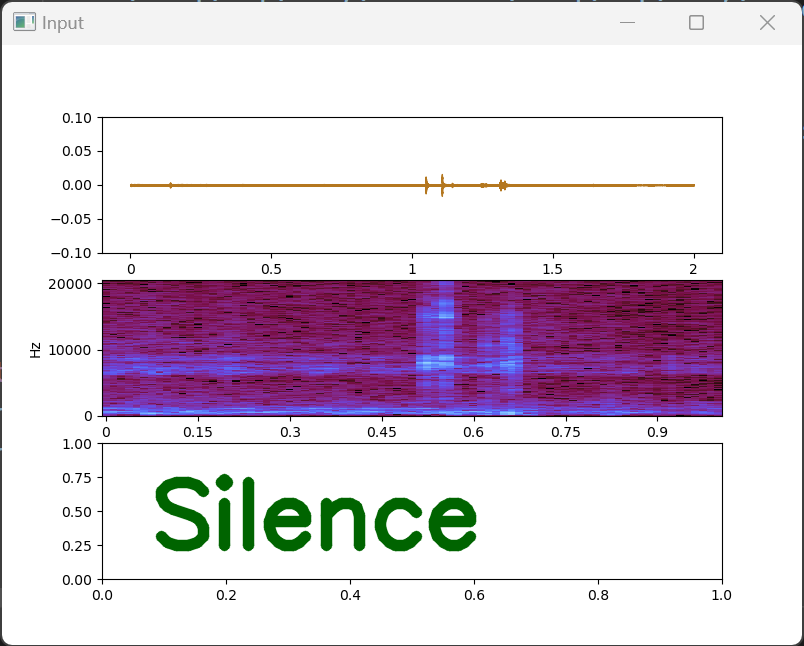
Note: In the entire process I just SVM model with default parameters (C=1.0, kernel=’rbf’, degree=3), but generally it’s a good practice to try several different machine learning models and choose the one which showed better results in terms of accuracy and generalization performance.
Leave a Reply