In the previous post, we have walked through the process of fitting a straight line or a polynomial line using linear regression on continues data. But, what if the output we are trying to predict is a discrete value. For example what if we are supposed to model a logical AND gate?!
In this case the modeling is quite a bit different. The underlying mechanics are basically the same as linear regression, but we should change the loss function, and also change the prediction in a way that it shows the probability of each possible output.
Sigmoid Function
As mentioned above, we still use the basics of the linear regression but this time, to be able to limit the predicted value between 0 and 1 which represents the probability of each output, we should pass the value of w*input to a function called Sigmoid or Logistic defined as:
import math
import matplotlib.pyplot as plt

def sigmoid(x):
    return 1.0/(1 + math.exp(-x))

x=[x * 0.1 for x in range(-100, 100)]
y=[sigmoid(x) for x in x]

plt.scatter(x, y)
plt.show()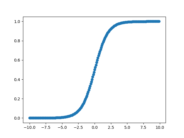
So let’s modify our linear regressor class and plug in the Sigmoid function in the predict() function as well.
import numpy as np
import math

def sigmoid(x):
    return 1/(1 + math.exp(-x))

class LogisticRegressor:
    """Logistic regression model"""
    def __init__(self, coeff=None):
        self.coeff = coeff

    def __add_bias(self, x):
        return np.append(x, 1)

    def predict(self, x):
        x = self.__add_bias(x)
        return sigmoid(self.coeff.dot(x.T))
Now, we can check the logistic regressor with arbitrary coefficients and the AND gate truth table as the prediction inputs.
model = LogisticRegressor(coeff=np.array([2.5,2.5,-4]))
x = np.array([[0,0],[0,1],[1,0],[1,1]])
predicted = [model.predict(input) for input in x ]
print(predicted))))
[0.01798620996209156, 0.18242552380635635, 0.18242552380635635, 0.7310585786300049]You may think that this result is not actual discrete 0, 1 value and you are right! but as we mentioned before, the output could be considered as the probability of the actual value being 1. Therefore, to work around it we should simply consider predicted values over a threshold to be 1 and values less than the threshold are 0.
threshold = 0.5
predicted = [1 if value > threshold else 0 for value in predicted]
print(predicted)
[0, 0, 0, 1]Cross-Entropy Loss Function
Just like the linear regression, in order to be able to assess the performance of our model, we need a measure of how good the model in predicting. In binary classification, Cross-Entropy loss function which is also called negative log likelihood does the job for us. This function is defined as below:
Leave a Reply